How to Understand the Bilateral Grid and Use It for Image Processing
0. Pre-word
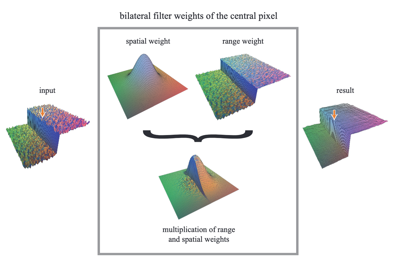
Bilateral Filter is a very famous denosing filter which not only could denoise and smooth the images but also could preserve the edge. The most easily understand illustration could be demonstrated as Fig 1. You could see from the illustration here, Bilateral Filter not only consider the spatial distance, but also will consider the pixel intensity distance. By that way, it could achieve edge-preserving denoising filter, which Gaussian filter cannot achieve.
So, the bilateral filter only with advantages but not disadvantages? The answer is No!!! Although the edge-presering property is really nice, however, since the nonlinearality inherent in the bilateral filter, it is very slow to implement bilateral filter. What is the Nonlinearality? Let’s compare bilateral filter with Gaussian filter, the Gaussian filter could be formulated as below:
\[I_{p}^{gf} = \frac{1}{W_{p}^{gf}}\sum_{q\in s}G_{s}(||p-q||_2^2)\cdot I_{q}\]where \(W_{p}^{gf}\) is the normalization constant;
And bilatera filter could be expressed as:
\[I_{p}^{bf} = \frac{1}{W_{p}^{bf}}\sum_{q\in s}G_s(||p-q||_2^2)\cdot {\color{red}G_r(|I_q - I_p|)} \cdot I_q\]where \(W_p^{bf}\) is the normalization constant as well.
\[W_p^{bf} = \sum_{q\in s}G_s(||p-q||_2^2)\cdot G_r(|I_q - I_p|)\]The most significant difference is point out by red text, which represent the filter not only take the spatial distance into account, but also will consider the intentsity diffenrence, the intensity difference too large, then the weight for that pixel will be very low! The nonlinearality comes from two aspects:
- The normalization constant, \(W_p^{bf}\);
-
The intensity weight part, $$G_r( I_q - I_p )$$;
Since they are directly related with pixel intensity.
Nonlinearality will result in what problems? The most severe part is about the running time of the filter; For normal Gaussian filter, we could pre-compute the convolution kernel as it only related to the relative spatial relationship, and for two-dimensional case, the 2D convolution could be seperated into two 1D convolution which could be accelerated by FFT algorithm;
1. Accelerating Bilateral Filter by Adding New Dimension
Strongly recommend reading the original paper: A Fast Approximation of the Bilateral Filter using a Signal Processing Approach by Sylvain Paris and Fr ́edo Durand;
The idea of this paper and method is so elegant from mathematical prospective, the core idea is “Adding a new dimension called range dimension, which represent the pixel range, for instance, 0-255 or 0.0-1.0, then treat the bilateral filter as a 3D convolution (for 2D images), two dimensions are spatial, the new dimension is range dimension”
Here is a 1D signal as example from the Jiawen Chen et,.al. The greatest part of this idea is by adding a new dimention, the edge are explicitly seperated in the new dimension, which make sure the edges will not be averaged during the concolution computing.
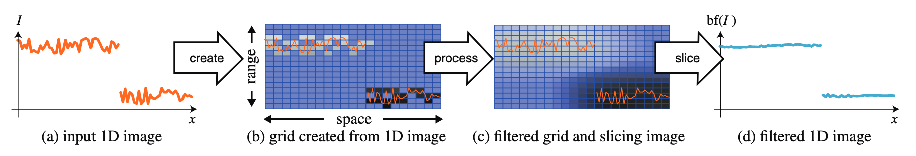
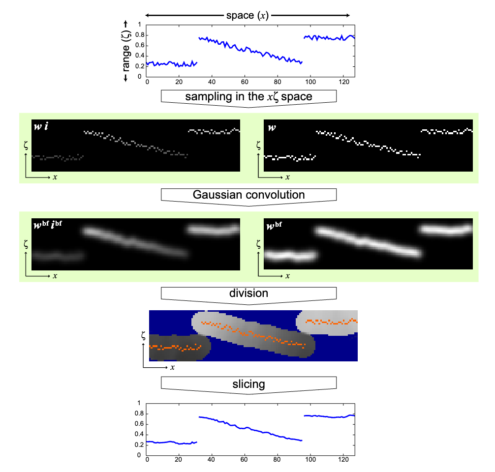
The basic procesures for this algorithms is shown in Fig 3. And you can see, we save a two-elements tuples in every grid, as we need to normalize the results.
One things I really want to share is the thread of development of: Bilateral Filter → Bilateral Grid. Till now, we just using adding a new dimension to accelerate the bilateral filter which works for denoise, however, when we talk about the bilateral grid, it represent a lot of local image operator, like style translation, denoising, and so many others image enhancement operators as shown in “Real-time Edge-Aware Image Processing with the Bilateral Grid”. Let’s continue dive in!
2. Bilateral Grid
In the paper “Real-time Edge-Aware Image Processing with the Bilateral Grid”, Jiawen Chen developed a new data structure, called Bilateral Grid, and they demonstrated by using Bilateral Grid, we could implement many image operators in a edge-preserve miner. The usage of this new data structure are listed below:
- Grid creation: in this stage, we initiate a grid and then to filling it;
- Processing: using any operators we need to processing the grid;
- Slicing: using the spatial and range index to get the processed results from the grid;
If you carefully look the Fig 2, you’ll find actually every single cell in the grid are not binary, but in the range dimension, for each pixel we only have a single pixel value, right? So, why it’s not binary? Here it comes! One of the advantages of using bilateral grid: the grid size could be way more smaller than the original size. For example, for an image with 720 * 1280 resolution, the resolution for bilateral grid could be much smaller, like 20 * 30, since the reducetion of resolution, the processing in bilateral grid instead of original input, will be much faster!
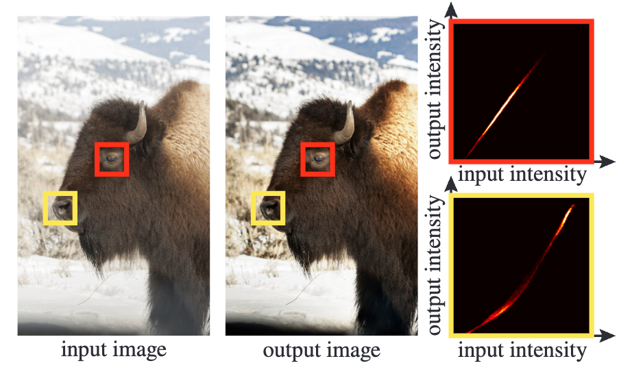
But you may be confued about that, why we could decrease the resolution of bilateral grid? Let me show you another nice paper from Jiawen Chen as well, “Bilateral Guided Upsampling”. In this paper, the authors have an observation: For most of image operators, the local patch will encounter an affine transformation. But you should remember, this is not mathematical proof, instead of apporximation, you could find the curve is not that straight.
Given that observation, we could understand why we could use lower resolution bilateral grid, since in certain local patch, these pixel processing could be very similar, even processed by a same affine transformation. More important, using bilateral grid not just process the spatial local patch, don’t forget we have a new range dimension! In the same cell of the bilateral grid, means in a local region no matter in Spatial or Pixel-range, which represent the same affine transformation only used when spatially and range closed to each other.
Thus, in the paper of “Bilateral Guided Upsampling”, the author demonstrate how to use the observation to implement some frequently used image operators by a faster way, shown in Fig 5.
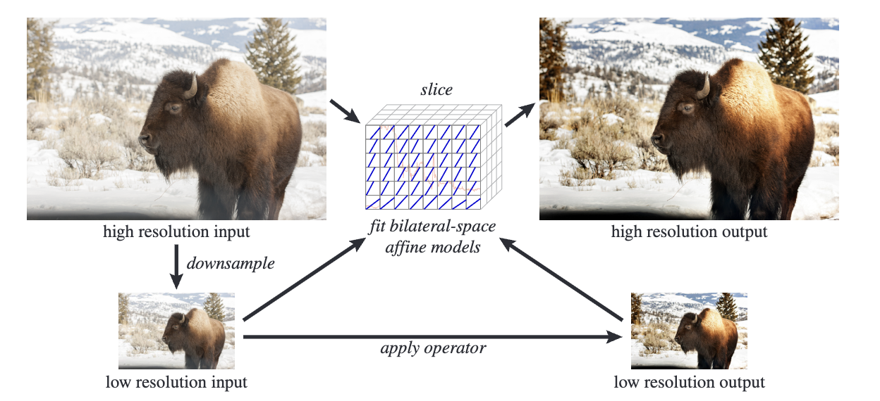
It’s easy and straight-forward to understand the Bilateral Grid now! We just to create a bilateral grid and then to put the original pixels into different cells by their spatial and range indices; for a certain cell, we use a same transformation to process the information; finally, we could using slicing to get the processed outputs.
In summary, bilateral grid is very useful to represent the local affine transformation category image operators and it’s very fast as it could be parallel by cuda or something else.
3. Bilateral Grid with Deep Learning
In this section, I would like to share a very famous and classical paper from Google and MIT, Deep Bilateral Learning for Real-Time Image Enhancement. This paper introduce bilateral grid into deep learning paradigm, overal pipeline see Fig 6.
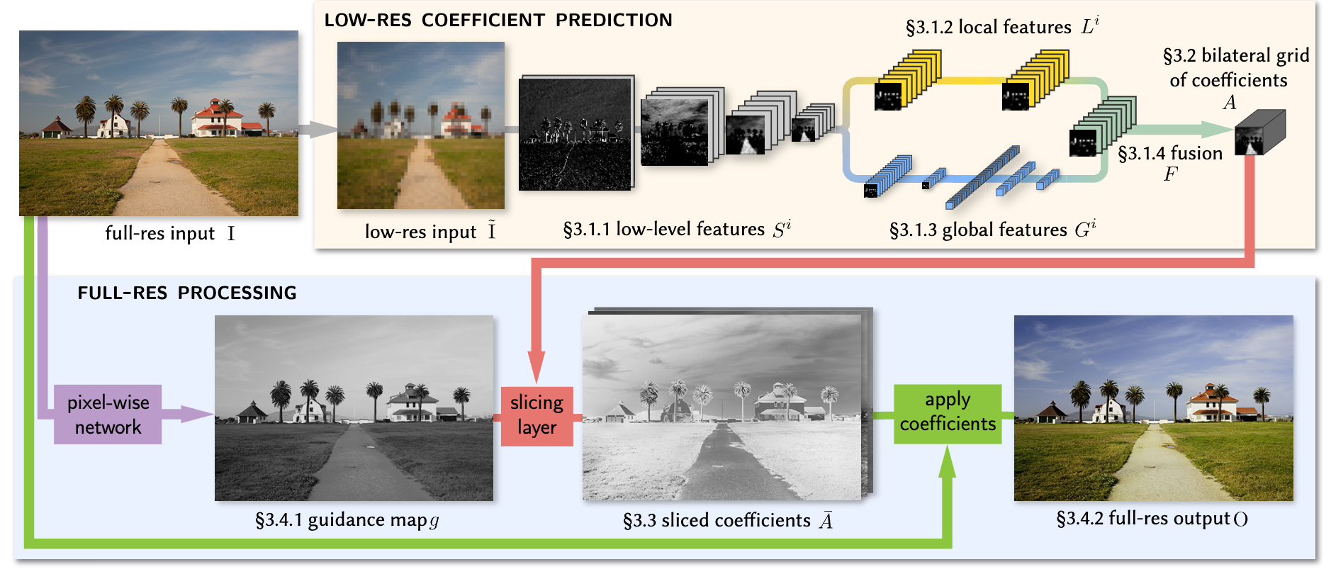
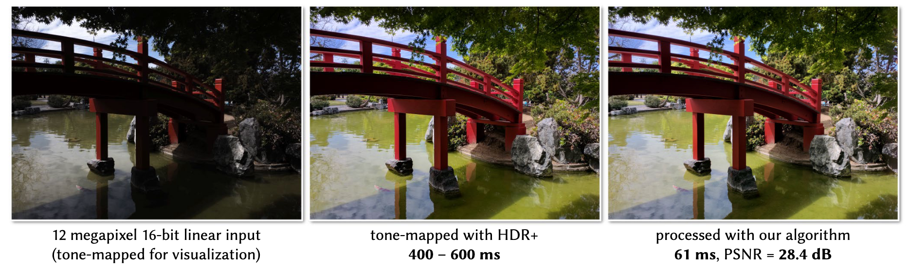
The most significant difference from the discussion above is this work using Learning to get the bilateral grid, even the bilateral grid itself is the learned features by neural networks. But the basic processures are keep the same! Since the use of bilateral grid like learning, the running speed is very competitive and it could run on mobile devices, like cellphones, Google actually depolied the algorithms on Google Pixel phones.
4. A Naive Implementation for Bilateral Grid
I will share the code in GitHub, please stay tune!